2 Data frames

Data frame is R’s name for tabular data. We generally want each row in a data frame to represent a unit of observation, and each column to contain a different type of information about the units of observation. Tabular data in this form is called “tidy data”.

Today we will be using a collection of modern packages collectively known as the Tidyverse. R and its predecessor S have a history dating back to 1976. The Tidyverse fixes some dubious design decisions baked into “base R”, including having its own slightly improved form of data frame, which is called a tibble. Sticking to the Tidyverse where possible is generally safer, Tidyverse packages are more willing to generate errors rather than ignore problems.

2.1 Setting up

Our first step is to download the files we need and to install the Tidyverse. This is the one step where we ask you to copy and paste some code:

# Download files for this workshop
download.file(
  "https://monashdatafluency.github.io/r-intro-2/r-intro-2-files.zip",
  destfile="r-intro-2-files.zip")
unzip("r-intro-2-files.zip")

# Install Tidyverse
install.packages("tidyverse")

If using RStudio Cloud, you might need to switch to R version 3.5.3 to successfully install Tidyverse. Use the drop-down in the top right corner of the page.

People also sometimes have problems installing all the packages in Tidyverse on Windows machines. If you run into problems you may have more success installing individual packages.

install.packages(c("dplyr","readr","tidyr","ggplot2"))

We need to load the tidyverse package in order to use it.

library(tidyverse)

# OR
library(dplyr)
library(readr)
library(tidyr)
library(ggplot2)

The tidyverse package loads various other packages, setting up a modern R environment. In this section we will be using functions from the dplyr, readr and tidyr packages.

R is a language with mini-languages within it that solve specific problem domains. dplyr is such a mini-language, a set of “verbs” (functions) that work well together. dplyr, with the help of tidyr for some more complex operations, provides a way to perform most manipulations on a data frame that you might need.

2.2 Loading data

We will use the read_csv function from readr to load a data set. (See also read.csv in base R.) CSV stands for Comma Separated Values, and is a text format used to store tabular data. The first few lines of the file we are loading are shown below. Conventionally the first line contains column headings.

name,region,oecd,g77,lat,long,income2017
Afghanistan,asia,FALSE,TRUE,33,66,low
Albania,europe,FALSE,FALSE,41,20,upper_mid
Algeria,africa,FALSE,TRUE,28,3,upper_mid
Andorra,europe,FALSE,FALSE,42.50779,1.52109,high
Angola,africa,FALSE,TRUE,-12.5,18.5,lower_mid

geo <- read_csv("r-intro-2-files/geo.csv")

## Rows: 196 Columns: 7
## ── Column specification ────────────────────────────────────────────────────────────────────────────────────────────────────
## Delimiter: ","
## chr (3): name, region, income2017
## dbl (2): lat, long
## lgl (2): oecd, g77
## 
## ℹ Use `spec()` to retrieve the full column specification for this data.
## ℹ Specify the column types or set `show_col_types = FALSE` to quiet this message.

geo

## # A tibble: 196 × 7
##    name                region   oecd  g77     lat   long income2017
##    <chr>               <chr>    <lgl> <lgl> <dbl>  <dbl> <chr>     
##  1 Afghanistan         asia     FALSE TRUE   33    66    low       
##  2 Albania             europe   FALSE FALSE  41    20    upper_mid 
##  3 Algeria             africa   FALSE TRUE   28     3    upper_mid 
##  4 Andorra             europe   FALSE FALSE  42.5   1.52 high      
##  5 Angola              africa   FALSE TRUE  -12.5  18.5  lower_mid 
##  6 Antigua and Barbuda americas FALSE TRUE   17.0 -61.8  high      
##  7 Argentina           americas FALSE TRUE  -34   -64    upper_mid 
##  8 Armenia             europe   FALSE FALSE  40.2  45    lower_mid 
##  9 Australia           asia     TRUE  FALSE -25   135    high      
## 10 Austria             europe   TRUE  FALSE  47.3  13.3  high      
## # … with 186 more rows

read_csv has guessed the type of data each column holds:

<chr> - character strings
<dbl> - numerical values. Technically these are “doubles”, which is a way of storing numbers with 15 digits precision.
<lgl> - logical values, TRUE or FALSE.

We will also encounter:

<int> - integers, a fancy name for whole numbers.
<fct> - factors, categorical data. We will get to this shortly.

You can also see this data frame referring to itself as “a tibble”. This is the Tidyverse’s improved form of data frame. Tibbles present themselves more conveniently than base R data frames. Base R data frames don’t show the type of each column, and output every row when you try to view them.

Tip

A data frame can also be created from vectors, with the tibble function. (See also data.frame in base R.) For example:

tibble(foo=c(10,20,30), bar=c("a","b","c"))

## # A tibble: 3 × 2
##     foo bar  
##   <dbl> <chr>
## 1    10 a    
## 2    20 b    
## 3    30 c

The argument names become column names in the data frame.

Tip

The path to the file on our server is "r-intro-2-files/geo.csv". This says, starting from your working directory, look in the directory r-intro-2-files for the file geo.csv. The steps in the path are separated by /. Your working directory is shown at the top of the console pane. The path needed might be different on your own computer, depending where you downloaded the file.

One way to work out the correct path is to find the file in the file browser pane, click on it and select “Import Dataset…”.

2.3 Exploring

The View function gives us a spreadsheet-like view of the data frame.

View(geo)

print with the n argument can be used to show more than the first 10 rows on the console.

print(geo, n=200)

We can extract details of the data frame with further functions:

nrow(geo)

## [1] 196

ncol(geo)

## [1] 7

colnames(geo)

## [1] "name"       "region"     "oecd"       "g77"        "lat"       
## [6] "long"       "income2017"

summary(geo)

##      name              region             oecd            g77         
##  Length:196         Length:196         Mode :logical   Mode :logical  
##  Class :character   Class :character   FALSE:165       FALSE:65       
##  Mode  :character   Mode  :character   TRUE :31        TRUE :131      
##                                                                       
##                                                                       
##                                                                       
##       lat              long           income2017       
##  Min.   :-42.00   Min.   :-175.000   Length:196        
##  1st Qu.:  4.00   1st Qu.:  -5.625   Class :character  
##  Median : 17.42   Median :  21.875   Mode  :character  
##  Mean   : 19.03   Mean   :  23.004                     
##  3rd Qu.: 39.82   3rd Qu.:  51.892                     
##  Max.   : 65.00   Max.   : 179.145

2.4 Indexing data frames

Data frames can be subset using [row,column] syntax.

geo[4,2]

## # A tibble: 1 × 1
##   region
##   <chr> 
## 1 europe

Note that while this is a single value, it is still wrapped in a data frame. (This is a behaviour specific to Tidyverse data frames.) More on this in a moment.

Columns can be given by name.

geo[4,"region"]

## # A tibble: 1 × 1
##   region
##   <chr> 
## 1 europe

The column or row may be omitted, thereby retrieving the entire row or column.

geo[4,]

## # A tibble: 1 × 7
##   name    region oecd  g77     lat  long income2017
##   <chr>   <chr>  <lgl> <lgl> <dbl> <dbl> <chr>     
## 1 Andorra europe FALSE FALSE  42.5  1.52 high

geo[,"region"]

## # A tibble: 196 × 1
##    region  
##    <chr>   
##  1 asia    
##  2 europe  
##  3 africa  
##  4 europe  
##  5 africa  
##  6 americas
##  7 americas
##  8 europe  
##  9 asia    
## 10 europe  
## # … with 186 more rows

Multiple rows or columns may be retrieved using a vector.

rows_wanted <- c(1,3,5)
geo[rows_wanted,]

## # A tibble: 3 × 7
##   name        region oecd  g77     lat  long income2017
##   <chr>       <chr>  <lgl> <lgl> <dbl> <dbl> <chr>     
## 1 Afghanistan asia   FALSE TRUE   33    66   low       
## 2 Algeria     africa FALSE TRUE   28     3   upper_mid 
## 3 Angola      africa FALSE TRUE  -12.5  18.5 lower_mid

Vector indexing can also be written on a single line.

geo[c(1,3,5),]

## # A tibble: 3 × 7
##   name        region oecd  g77     lat  long income2017
##   <chr>       <chr>  <lgl> <lgl> <dbl> <dbl> <chr>     
## 1 Afghanistan asia   FALSE TRUE   33    66   low       
## 2 Algeria     africa FALSE TRUE   28     3   upper_mid 
## 3 Angola      africa FALSE TRUE  -12.5  18.5 lower_mid

geo[1:7,]

## # A tibble: 7 × 7
##   name                region   oecd  g77     lat   long income2017
##   <chr>               <chr>    <lgl> <lgl> <dbl>  <dbl> <chr>     
## 1 Afghanistan         asia     FALSE TRUE   33    66    low       
## 2 Albania             europe   FALSE FALSE  41    20    upper_mid 
## 3 Algeria             africa   FALSE TRUE   28     3    upper_mid 
## 4 Andorra             europe   FALSE FALSE  42.5   1.52 high      
## 5 Angola              africa   FALSE TRUE  -12.5  18.5  lower_mid 
## 6 Antigua and Barbuda americas FALSE TRUE   17.0 -61.8  high      
## 7 Argentina           americas FALSE TRUE  -34   -64    upper_mid

2.5 Columns are vectors

Ok, so how do we actually get data out of a data frame?

Under the hood, a data frame is a list of column vectors. We can use $ to retrieve columns. Occasionally it is also useful to use [[ ]] to retrieve columns, for example if the column name we want is stored in a variable.

head( geo$region )

## [1] "asia"     "europe"   "africa"   "europe"   "africa"   "americas"

head( geo[["region"]] )

## [1] "asia"     "europe"   "africa"   "europe"   "africa"   "americas"

To get the “region” value of the 4th row as above, but unwrapped, we can use:

geo$region[4]

## [1] "europe"

For example, to plot the longitudes and latitudes we could use:

plot(geo$long, geo$lat)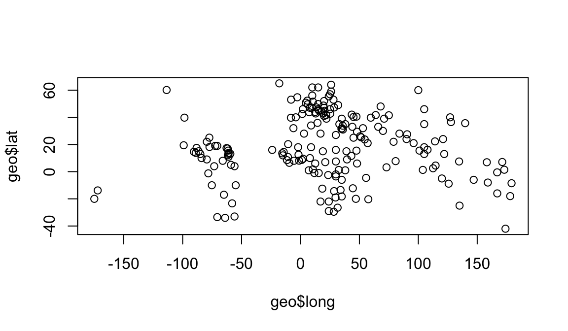

Quiz: reading R code

You encounter some wild R code, and aren’t sure what it does. Based on R syntax you’ve encountered so far, what roles are the different names in this code playing?

highest <- geo$name[ head(order(geo$lat, decreasing=TRUE), n=10) ]

Find all examples of:

A. The name of a variable to store a value to.
B. The name of a variable to retrieve the value from.
C. The name of a column to get from a data frame.
D. The name of a function to call.
E. The name of an argument to a function call.

See here for answers.

2.6 Logical indexing

A method of indexing that we haven’t discussed yet is logical indexing. Instead of specifying the row number or numbers that we want, we can give a logical vector which is TRUE for the rows we want and FALSE otherwise. This can also be used with vectors.

We will first do this in a slightly verbose way in order to understand it, then learn a more concise way to do this using the dplyr package.

Southern countries have latitude less than zero.

is_southern <- geo$lat < 0

head(is_southern)

## [1] FALSE FALSE FALSE FALSE  TRUE FALSE

sum(is_southern)

## [1] 40

sum treats TRUE as 1 and FALSE as 0, so it tells us the number of TRUE elements in the vector.

We can use this logical vector to get the southern countries from geo:

geo[is_southern,]

## # A tibble: 40 × 7
##    name             region   oecd  g77     lat  long income2017
##    <chr>            <chr>    <lgl> <lgl> <dbl> <dbl> <chr>     
##  1 Angola           africa   FALSE TRUE  -12.5  18.5 lower_mid 
##  2 Argentina        americas FALSE TRUE  -34   -64   upper_mid 
##  3 Australia        asia     TRUE  FALSE -25   135   high      
##  4 Bolivia          americas FALSE TRUE  -17   -65   lower_mid 
##  5 Botswana         africa   FALSE TRUE  -22    24   upper_mid 
##  6 Brazil           americas FALSE TRUE  -10   -55   upper_mid 
##  7 Burundi          africa   FALSE TRUE   -3.5  30   low       
##  8 Chile            americas TRUE  TRUE  -33.5 -70.6 high      
##  9 Comoros          africa   FALSE TRUE  -12.2  44.4 low       
## 10 Congo, Dem. Rep. africa   FALSE TRUE   -2.5  23.5 low       
## # … with 30 more rows

Comparison operators available are:

x == y – “equal to”
x != y – “not equal to”
x < y – “less than”
x > y – “greater than”
x <= y – “less than or equal to”
x >= y – “greater than or equal to”

More complicated conditions can be constructed using logical operators:

a & b – “and”, TRUE only if both a and b are TRUE.
a | b – “or”, TRUE if either a or b or both are TRUE.
! a – “not” , TRUE if a is FALSE, and FALSE if a is TRUE.

The oecd column of geo tells which countries are in the Organisation for Economic Co-operation and Development, and the g77 column tells which countries are in the Group of 77 (an alliance of developing nations). We could see which OECD countries are in the southern hemisphere with:

southern_oecd <- is_southern & geo$oecd

geo[southern_oecd,]

## # A tibble: 3 × 7
##   name        region   oecd  g77     lat  long income2017
##   <chr>       <chr>    <lgl> <lgl> <dbl> <dbl> <chr>     
## 1 Australia   asia     TRUE  FALSE -25   135   high      
## 2 Chile       americas TRUE  TRUE  -33.5 -70.6 high      
## 3 New Zealand asia     TRUE  FALSE -42   174   high

is_southern seems like it should be kept within our geo data frame for future use. We can add it as a new column of the data frame with:

geo$southern <- is_southern

geo

## # A tibble: 196 × 8
##    name                region   oecd  g77     lat   long income2017 southern
##    <chr>               <chr>    <lgl> <lgl> <dbl>  <dbl> <chr>      <lgl>   
##  1 Afghanistan         asia     FALSE TRUE   33    66    low        FALSE   
##  2 Albania             europe   FALSE FALSE  41    20    upper_mid  FALSE   
##  3 Algeria             africa   FALSE TRUE   28     3    upper_mid  FALSE   
##  4 Andorra             europe   FALSE FALSE  42.5   1.52 high       FALSE   
##  5 Angola              africa   FALSE TRUE  -12.5  18.5  lower_mid  TRUE    
##  6 Antigua and Barbuda americas FALSE TRUE   17.0 -61.8  high       FALSE   
##  7 Argentina           americas FALSE TRUE  -34   -64    upper_mid  TRUE    
##  8 Armenia             europe   FALSE FALSE  40.2  45    lower_mid  FALSE   
##  9 Australia           asia     TRUE  FALSE -25   135    high       TRUE    
## 10 Austria             europe   TRUE  FALSE  47.3  13.3  high       FALSE   
## # … with 186 more rows

Challenge: logical indexing

Which country is in both the OECD and the G77?
Which countries are in neither the OECD nor the G77?
Which countries are in the Americas? These have longitudes between -150 and -40.

2.6.1 A `dplyr` shorthand

The above method is a little laborious. We have to keep mentioning the name of the data frame, and there is a lot of punctuation to keep track of. dplyr provides a slightly magical function called filter which lets us write more concisely. For example:

filter(geo, lat < 0 & oecd)

## # A tibble: 3 × 8
##   name        region   oecd  g77     lat  long income2017 southern
##   <chr>       <chr>    <lgl> <lgl> <dbl> <dbl> <chr>      <lgl>   
## 1 Australia   asia     TRUE  FALSE -25   135   high       TRUE    
## 2 Chile       americas TRUE  TRUE  -33.5 -70.6 high       TRUE    
## 3 New Zealand asia     TRUE  FALSE -42   174   high       TRUE

In the second argument, we are able to refer to columns of the data frame as though they were variables. The code is beautiful, but also opaque. It’s important to understand that under the hood we are creating and combining logical vectors.

2.7 Factors

The count function from dplyr can help us understand the contents of some of the columns in geo. count is also magical, we can refer to columns of the data frame directly in the arguments to count.

count(geo, region)

## # A tibble: 4 × 2
##   region       n
##   <chr>    <int>
## 1 africa      54
## 2 americas    35
## 3 asia        59
## 4 europe      48

count(geo, income2017)

## # A tibble: 4 × 2
##   income2017     n
##   <chr>      <int>
## 1 high          58
## 2 low           31
## 3 lower_mid     52
## 4 upper_mid     55

One annoyance here is that the different categories in income2017 aren’t in a sensible order. This comes up quite often, for example when sorting or plotting categorical data. R’s solution is a further type of vector called a factor (think a factor of an experimental design). A factor holds categorical data, and has an associated ordered set of levels. It is otherwise quite similar to a character vector.

Any sort of vector can be converted to a factor using the factor function. This function defaults to placing the levels in alphabetical order, but takes a levels argument that can override this.

head( factor(geo$income2017, levels=c("low","lower_mid","upper_mid","high")) )

## [1] low       upper_mid upper_mid high      lower_mid high     
## Levels: low lower_mid upper_mid high

We should modify the income2017 column of the geo table in order to use this:

geo$income2017 <- factor(geo$income2017, levels=c("low","lower_mid","upper_mid","high"))

count now produces the desired order of output:

count(geo, income2017)

## # A tibble: 4 × 2
##   income2017     n
##   <fct>      <int>
## 1 low           31
## 2 lower_mid     52
## 3 upper_mid     55
## 4 high          58

When plot is given a factor, it shows a bar plot:

plot(geo$income2017)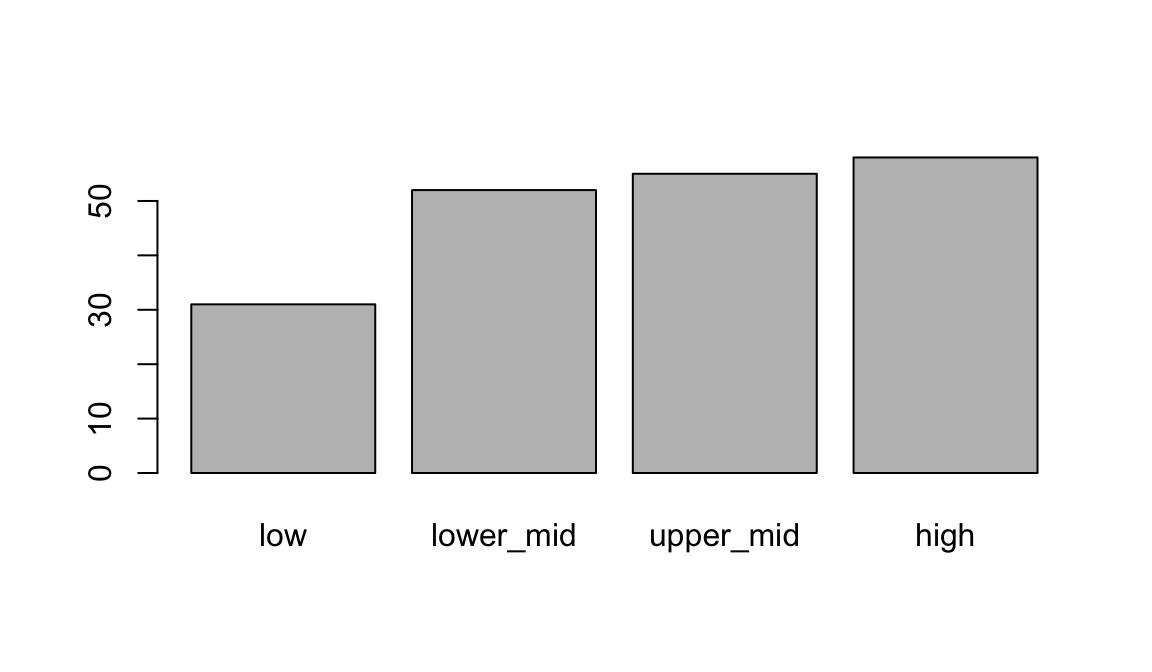

When given two factors, it shows a mosaic plot:

plot(geo$income2017, factor(geo$oecd))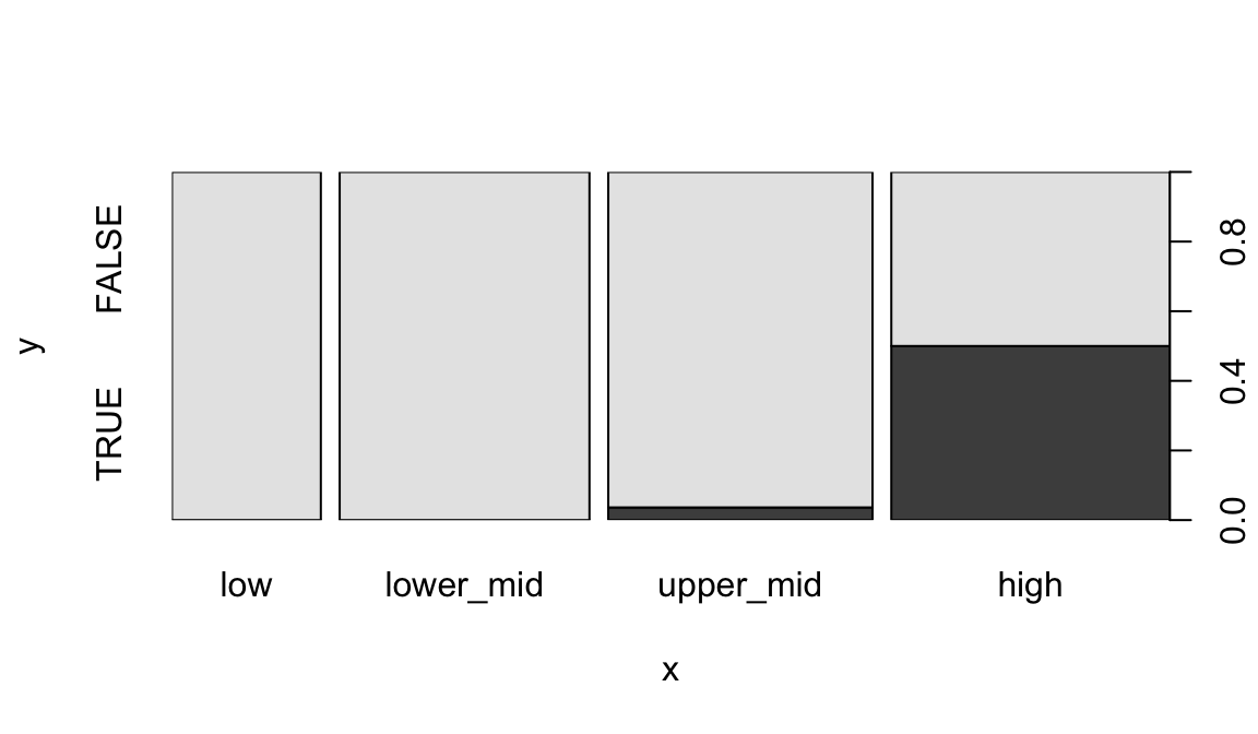

Similarly we can count two categorical columns at once.

count(geo, income2017, oecd)

## # A tibble: 6 × 3
##   income2017 oecd      n
##   <fct>      <lgl> <int>
## 1 low        FALSE    31
## 2 lower_mid  FALSE    52
## 3 upper_mid  FALSE    53
## 4 upper_mid  TRUE      2
## 5 high       FALSE    29
## 6 high       TRUE     29

2.8 Readability vs tidyness

The counts we obtained counting income2017 vs oecd were properly tidy in the sense of containing a single unit of observation per row. However to view the data, it would be more convenient to have income as columns and OECD membership as rows. We can use the pivot_wider function from tidyr to achieve this. (This is also sometimes also called a “cast” or a “spread”.)

counts <- count(geo, income2017, oecd)
pivot_wider(counts, names_from=income2017, values_from=n)

## # A tibble: 2 × 5
##   oecd    low lower_mid upper_mid  high
##   <lgl> <int>     <int>     <int> <int>
## 1 FALSE    31        52        53    29
## 2 TRUE     NA        NA         2    29

We could further specify values_fill=list(n=0) to fill in the NA values with 0. Or when using count, make sure all the relevant columns are factors and specify .drop=FALSE.

Tip

Tidying is often the first step when exploring a data-set. The tidyr package contains a number of useful functions that help tidy (or un-tidy!) data. We’ve just seen pivot_wider which spreads two columns into multiple columns. The inverse of pivot_wider is pivot_longer, which gathers multiple columns into two columns: a column of column names, and a column of values. pivot_longer is often the first step when tidying a dataset you have received from the wild. (This is sometimes also called a “melt” or a “gather”.)

Challenge: counting

Investigate how many OECD and non-OECD nations come from the northern and southern hemispheres.

Using count.
By making a mosaic plot.

Remember you may need to convert columns to factors for plot to work, and that a southern column could be added to geo with:

geo$southern <- geo$lat < 0

2.9 Sorting

Data frames can be sorted using the arrange function in dplyr.

arrange(geo, lat)

## # A tibble: 196 × 8
##    name         region   oecd  g77     lat  long income2017 southern
##    <chr>        <chr>    <lgl> <lgl> <dbl> <dbl> <fct>      <lgl>   
##  1 New Zealand  asia     TRUE  FALSE -42   174   high       TRUE    
##  2 Argentina    americas FALSE TRUE  -34   -64   upper_mid  TRUE    
##  3 Chile        americas TRUE  TRUE  -33.5 -70.6 high       TRUE    
##  4 Uruguay      americas FALSE TRUE  -33   -56   high       TRUE    
##  5 Lesotho      africa   FALSE TRUE  -29.5  28.2 lower_mid  TRUE    
##  6 South Africa africa   FALSE TRUE  -29    24   upper_mid  TRUE    
##  7 Swaziland    africa   FALSE TRUE  -26.5  31.5 lower_mid  TRUE    
##  8 Australia    asia     TRUE  FALSE -25   135   high       TRUE    
##  9 Paraguay     americas FALSE TRUE  -23.3 -58   upper_mid  TRUE    
## 10 Botswana     africa   FALSE TRUE  -22    24   upper_mid  TRUE    
## # … with 186 more rows

Numeric columns are sorted in numeric order. Character columns will be sorted in alphabetical order. Factor columns are sorted in order of their levels. The desc helper function can be used to sort in descending order.

arrange(geo, desc(name))

## # A tibble: 196 × 8
##    name           region   oecd  g77     lat   long income2017 southern
##    <chr>          <chr>    <lgl> <lgl> <dbl>  <dbl> <fct>      <lgl>   
##  1 Zimbabwe       africa   FALSE TRUE  -19    29.8  low        TRUE    
##  2 Zambia         africa   FALSE TRUE  -14.3  28.5  lower_mid  TRUE    
##  3 Yemen          asia     FALSE TRUE   15.5  47.5  lower_mid  FALSE   
##  4 Vietnam        asia     FALSE TRUE   16.2 108.   lower_mid  FALSE   
##  5 Venezuela      americas FALSE TRUE    8   -66    upper_mid  FALSE   
##  6 Vanuatu        asia     FALSE TRUE  -16   167    lower_mid  TRUE    
##  7 Uzbekistan     asia     FALSE FALSE  41.7  63.8  lower_mid  FALSE   
##  8 Uruguay        americas FALSE TRUE  -33   -56    high       TRUE    
##  9 United States  americas TRUE  FALSE  39.8 -98.5  high       FALSE   
## 10 United Kingdom europe   TRUE  FALSE  54.8  -2.70 high       FALSE   
## # … with 186 more rows

2.10 Joining data frames

Let’s move on to a larger data set. This is from the Gapminder project and contains information about countries over time.

gap <- read_csv("r-intro-2-files/gap-minder.csv")
gap

## # A tibble: 4,312 × 5
##    name                 year population gdp_percap life_exp
##    <chr>               <dbl>      <dbl>      <dbl>    <dbl>
##  1 Afghanistan          1800    3280000        603     28.2
##  2 Albania              1800     410445        667     35.4
##  3 Algeria              1800    2503218        715     28.8
##  4 Andorra              1800       2654       1197     NA  
##  5 Angola               1800    1567028        618     27.0
##  6 Antigua and Barbuda  1800      37000        757     33.5
##  7 Argentina            1800     534000       1507     33.2
##  8 Armenia              1800     413326        514     34  
##  9 Australia            1800     351014        814     34.0
## 10 Austria              1800    3205587       1847     34.4
## # … with 4,302 more rows

Quiz

What is the unit of observation in this new data frame?

It would be useful to have general information about countries from geo available as columns when we use this data frame. gap and geo share a column called name which can be used to match rows from one to the other.

gap_geo <- left_join(gap, geo, by="name")
gap_geo

## # A tibble: 4,312 × 12
##    name     year popul…¹ gdp_p…² life_…³ region oecd  g77     lat   long incom…⁴
##    <chr>   <dbl>   <dbl>   <dbl>   <dbl> <chr>  <lgl> <lgl> <dbl>  <dbl> <fct>  
##  1 Afghan…  1800 3280000     603    28.2 asia   FALSE TRUE   33    66    low    
##  2 Albania  1800  410445     667    35.4 europe FALSE FALSE  41    20    upper_…
##  3 Algeria  1800 2503218     715    28.8 africa FALSE TRUE   28     3    upper_…
##  4 Andorra  1800    2654    1197    NA   europe FALSE FALSE  42.5   1.52 high   
##  5 Angola   1800 1567028     618    27.0 africa FALSE TRUE  -12.5  18.5  lower_…
##  6 Antigu…  1800   37000     757    33.5 ameri… FALSE TRUE   17.0 -61.8  high   
##  7 Argent…  1800  534000    1507    33.2 ameri… FALSE TRUE  -34   -64    upper_…
##  8 Armenia  1800  413326     514    34   europe FALSE FALSE  40.2  45    lower_…
##  9 Austra…  1800  351014     814    34.0 asia   TRUE  FALSE -25   135    high   
## 10 Austria  1800 3205587    1847    34.4 europe TRUE  FALSE  47.3  13.3  high   
## # … with 4,302 more rows, 1 more variable: southern <lgl>, and abbreviated
## #   variable names ¹population, ²gdp_percap, ³life_exp, ⁴income2017

The output contains all ways of pairing up rows by name. In this case each row of geo pairs up with multiple rows of gap.

The “left” in “left join” refers to how rows that can’t be paired up are handled. left_join keeps all rows from the first data frame but not the second. This is a good default when the intent is to attaching some extra information to a data frame. inner_join discards all rows that can’t be paired up. full_join keeps all rows from both data frames.

2.11 Further reading

We’ve covered the fundamentals of dplyr and data frames, but there is much more to learn. Notably, we haven’t covered the use of the pipe %>% to chain dplyr verbs together. The “R for Data Science” book is an excellent source to learn more. The Monash Data Fluency “Programming and Tidy data analysis in R” course also covers this.